Covering Spaces of a Robot Arm's Flat Torus C-Space

Consider a double-pendulum robot arm with c-space a 2D torus \(T^2\).

A 2D robot arm
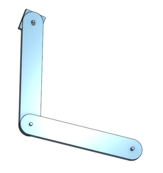
My CAD model of a 2D pendulum (click for OnShape link)

3D printed robot arm
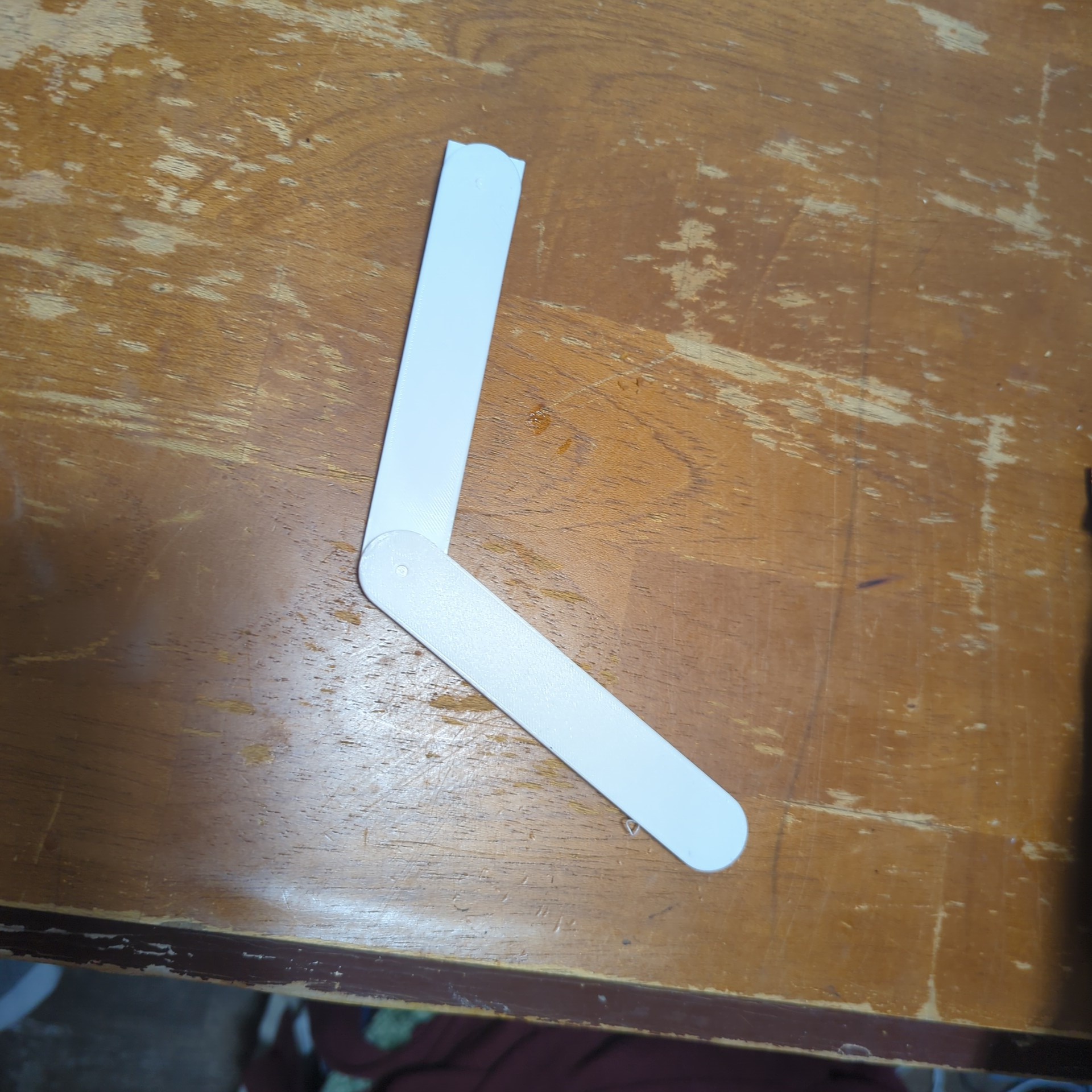
My 3D print of my 2D CAD model

Torus c-space
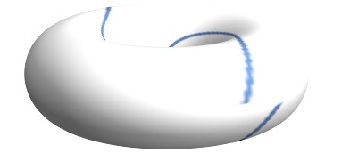
The 2D c-space of my double pendulum CAD model with a (not closed) geodesic traced out on it


A video of Prof. Jim Yorke displaying chaotic properties of the double pendulum at a Mardem lecture at UWM.


A video of Prof. Steve Brunton displaying control engineering of the chaos on the double pendulum.


A video of a Boston Dynamics robot dancing.
(When on can "make the system dance" [usually metaprhorical, but literal in this case], one generally has the desired level of control of the system.)

We shall identify \(T^2\) with \([0,2\pi]^2\), with units of radians, via the standard coordinate patch \(\phi: [0, 2\pi]^2 \to T^2\) given by \(\phi(\theta_1, \theta_2) = ((\cos(\theta_1), \sin(\theta_1)), (\cos(\theta_2), \sin(\theta_1)))\) and therefore endow it with the 
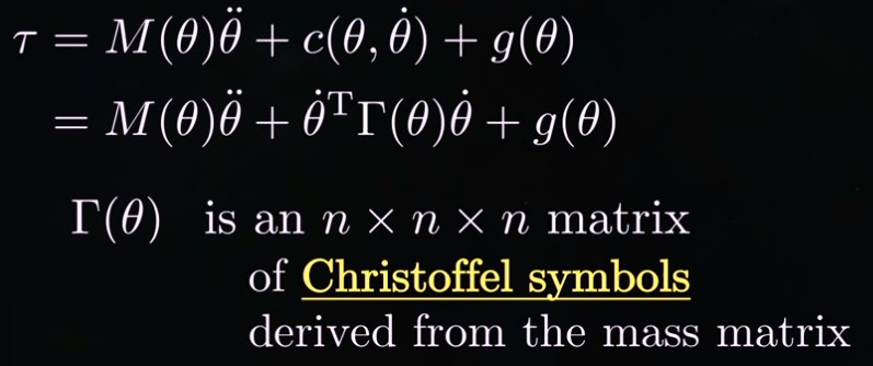
units of radians, although it is technically unitless. The Riemannian metric (r-metric) \(g(\theta_1, \theta_2)\) (written as \(M(\theta)\) in the following graphic from https://youtu.be/BjD-pL819LA?si=q8_It-jJFEq0AmEu&t=212; \(g(\theta)\) in the following graphic is the gravity term) may be read off the equation of motion (EoM):

Equation of Motion for motion on a 2-torus

The Riemannian metric in the standard coordinate patch for this robot arm is given by

\[ g(\theta_1,\theta_2) = \begin{bmatrix} [I_{zz,1} + I_{zz,2} + (L_1^2m_1)/4 + L_1^2m_2 + (L_2^2m_2)/4 + L_1L_2m_2\cos(\theta_2) & (m_2L_2^2)/4 + (L_1L_2m_2\cos(\theta_2))/2 + I_{zz,2} \\
(m_2L_2^2)/4 + (L_1L_2m_2\cos(\theta_2))/2 + I_{zz,2} &                            (m_2L_2^2)/4 + I_{zz,2}\\ \end{bmatrix} \]

(For definiteness, for this particular double-pendulum robot arm, the values of the parameters are  \(m_i = 28.927\) kg, \(I_{zz,i} = 3.335\) \(\text{kg}\cdot\text{m}^2\), and \(L_i = 1.000\) m in SI, but these values are mutable. Here is an OnShape model of the robot arm https://cad.onshape.com/documents/13c5b197f578ed74e3c43266/w/31eaf96cbef839c27d1f6215/e/2af3572176e096bf67365da2?renderMode=0&uiState=64c22d4a8c079b328fbabd57. Using these values leads to a r-metric of


\[g(\theta_1, \theta_2) = \begin{bmatrix} 28.927\cos(\theta_2) + 50.06 & 14.463\cos(\theta_2) + 10.567 \\
14.463\cos(\theta_2) + 10.567 &                      10.567\end{bmatrix}.)\]

Note that the entries in the Riemannian metric have dimensions of \(\left[\text{Length}^2 \cdot \text{Mass}\right]\). (It should be noted that there are dimensions/units used for the describing the robot arm and hence, perhaps bizarrely, for describing the Riemannian metric. Points in the manifold and tangent vectors to the manifold are part of the intrinsic topology of the underlying smooth manifold of the c-space and have only dimensions of [Angular Measure], while inner products/norms of tangent vectors and lengths of curves/distances between points in the manifold depend on Riemannian metric, which is extrinsic to the topology of the underlying manifold; inner products of tangent vectors have dimensions of \(\displaystyle\left[\text{Angular Measure}^2\cdot\text{Length}^2 \cdot \text{Mass}\right]\) while norms of tangent vectors and lengths of curves/distances between points have units of \(\displaystyle\left[\text{Angular Measure}\cdot\text{Length} \cdot \text{Mass}^{\frac{1}{2}}\right]\).)

This link I think I computes the sectional curvature correctly in MATLAB, and it is identically 0. This link (shamelessly pirated from [1]) I think confirms the computation of the sectional curvature of my Riemannian manifold in Mathematica (although it heavily uses the fact we are in dimension 2; I'll need to work on that). This link shows that the volume of the torus is 693.121 \(\left[\text{rad}^2\cdot\text{m}^2\cdot\text{kg}\right]\)

First, let us consider the infimum of path lengths metric \(\left(\text{in }\displaystyle\left[\text{rad}\cdot\text{m} \cdot \text{kg}^{\frac{1}{2}}\right]\right)\) on \((T^2,g)\) itself. (NB: This is per a discussion with Boris Okun on 08/10/2023.)

Next, let us consider the "standard" loop based at (0,0) that goes around the "first" circle of the torus rel endpoints. This loop may be homotoped rel its endpoints to the shortest path in its homotopy class rel endpoints; by the argument in [4] and its second comment, this second loop should be the unique geodesic in this homotopy class. Consider the tangent vector at the origin, \(\vec{v}_1\), with the property that the geodesic associated to \(\vec{v}_1\) goes around this second loop, a geodesic, from \(t=0\) to \(t=1\). In a similar way, form a second tangent vector \(\vec{v}_2\) at the origin so that the geodesic based at (0,0) that is homotopic to the "second" circle of the torus rel endpoints associated to this tangent vector goes around once from \(t=0\) to \(t=1\). Call this first lattice \(\Lambda_1 = (\vec{v}_1, \vec{v}_2)\)

Continuing, consider the tangent space at \((0,0)\) to \((\mathbb{R}^2, i)\), with its standard Riemannian metric. Form the lattice \(\Lambda_2 = (\vec{w}_1, \vec{w}_2)\) having \(\vec{w}_1 = ||\vec{v}_1||\hat{i}\) and having \(\vec{w}_2\) with the same norm as \(\vec{v}_2\), the same unordered angle with \(\vec{w}_1\) that \(\vec{v}_1\) has with \(\vec{v}_2\), and pointing in the upper-half plane (UHP).

A Straightening-Up Lemma Of Sorts: By [6], according to the Cartan-Hadamard Theorem, each tangent space at the identity, together with the exponential map, is the universal cover of its associated torus. But, of course, any two simply-connected covering spaces (with covering maps) are canonically homeomorphic (diffeomorphic, indeed, isometric, in fact, in this case)! In particular, by [3] and [6], there is an isometry \(f\) which goes from \((T^2, g)\) to a "straight" flat torus using a lattice \(\Lambda_2\) and a parallelogram in \(\mathbb{R}^2\) formed by using the two exponential maps, sending \(\exp_1(t_1\vec{v}_1 +t_2\vec{v}_2)\) to \(\exp_2(t_2\vec{w}_1 + t_2\vec{w}_2)\).

This leads to a commutative diagram of covering spaces

\[\begin{array}{ccc}  
T_{(0,0)}(T^2)\ \left[\text{rad}\right]                   & \xrightarrow{\cong, \tilde{f}} & T_{(0,0)}(T^2)\ \left[\text{rad}\right]                                                             \\

\downarrow (\exp_1)                                              &                                              & \downarrow (\exp_2)                                                            \\

(T^2,g)\ \left(\left[\text{rad}\right],\left[\text{m}^2\cdot\text{kg}\right]\right) &  \xrightarrow{\cong, f}           & (T_{(0,0)}(T^2)/\Lambda_2, i)\ ([\text{rad}],[\text{m}^2 \cdot \text{kg}])\ \text{("Straight Flat Torus")} \\
\end{array}\]

The problem now is to identify \(\Lambda_1\), that is, to identify the two smallest-length closed geodesics emanating from \((0,0)\) [rad] in \((T^2,g)\) with winding numbers (1,0) and (0,1) respectively, their unit tangent vectors, and the geodesics' lengths.

Since \(g\) is independent of \(\theta_1\), \(\gamma_1:\ [0,2\pi] \to T^2\) given by \(\gamma_1(t) = (t,0)\) should be a geodesic (\(t\) is a unitless parameter). Hence, if \(C_1\) is the closed curve corresponding to \(\gamma_1\), we should have  \(\displaystyle L(C_1) = \oint\limits_{C_1}\ 1\ ds = \int\limits_0^{2\pi} 1||\hat{\theta}_1||\ dt = \int\limits_0^{1} 2\pi||\hat{\theta}_1||\ dt' = \int\limits_0^{1} 2\pi\left(\sqrt{\hat{\theta}_1^T g\hat{\theta}_1}\right)\ dt' = \int\limits_0^{1} 2\pi(8.887)\ dt' = 55.842\ \left[\text{rad}\cdot\text{m} \cdot \text{kg}^{\frac{1}{2}}\right]\). So, we should have \(\displaystyle \vec{v}_1 = 2\pi\hat{\theta}_1\ \left(\text{norm has units of }\left[\text{rad}\cdot\text{m} \cdot \text{kg}^{\frac{1}{2}}\right]\right)\), and \(\displaystyle\vec{w}_1 = 55.842\hat{i}\ \left(\text{norm has units of }\left[\text{rad}\cdot\text{m} \cdot \text{kg}^{\frac{1}{2}}\right]\right)\).

Finding the other tangent vector \(\vec{v}_2\) would involve finding the second geodesic. This would involve starting with the path \(\gamma_4:\ [0, 2\pi] \to T^2\) given by \(\gamma_4(t) = ((1,0),(\\cos(t), \sin(t))\) and use the Calculus of Variations to find the variation on its homotopy class rel endpoints, \(\gamma_5(t) = (\cos[\eta(t)], \sin[\eta(t)]]), (\cos(t), \sin(t))\) minimizing the length in MATLAB or Python (see [7]), integrating the unitless scalar function 1 over the closed curve \(C_4\) associated to \(\gamma_5\) with respect to arc length to get the geodesic's length, and reparameterizing \(\gamma_5\) to \(\gamma_6\) whose domain is [0, 1]; then \(\displaystyle\vec{v}_2 = \left.\frac{d\gamma_6}{dt}\right|^{t=0}\).

The Calculus of Variations problem is to minimize \(\displaystyle J[\eta(t)] = \int\limits_0^{2\pi} \left|\left|\frac{d\gamma_5}{dt}\right|\right|\ dt = \int\limits_0^{2\pi} ||\eta'(t)\hat{\eta(t)}_1 + 1\hat{t}_2||\ dt = \int\limits_0^{2\pi} \left(\sqrt{[\eta'(t)\hat{\eta(t)}_1 + 1\hat{t}_2]^T\begin{bmatrix} 28.927\cos(t) + 50.06 & 14.463\cos(t) + 10.567 \\ 14.463\cos(t) + 10.567 & 10.567\end{bmatrix}[\eta'(t)\hat{\eta(t)}_1 + 1\hat{t}_2]}\right)\ dt\) subject to \(\eta(0) = \eta(2\pi) = 0\).

The Calculus of Variations problem is solved by setting \(\displaystyle L(t, s, s') = \sqrt{[s'\hat{\eta(t)}_1 + 1\hat{t}_2]^T\begin{bmatrix} 28.927\cos(t) + 50.06 & 14.463\cos(t) + 10.567 \\ 14.463\cos(t) + 10.567 & 10.567\end{bmatrix}[s'\hat{\eta(t)}_1 + 1\hat{t}_2]}\) and solving \(\displaystyle \frac{\partial}{\partial t}\left\{\frac{\partial L}{\partial s'}\right\} = 0\).

This MATLAB script appears to show there is no (real, nonzero) solution to the Calculus of Variations problem. If this is the case, then \(\eta(t) \equiv 0\) and \(\displaystyle \vec{v}_2 = 2\pi\hat{\theta}_1\ \left(\text{norm has units of }\left[\text{rad}\cdot\text{m} \cdot \text{kg}^{\frac{1}{2}}\right]\right)\), so that \(||\vec{w}_2||\) is 20.425 \(\left[\text{rad}\cdot\text{m} \cdot \text{kg}^{\frac{1}{2}}\right]\) and the angle between \(\vec{w}_1\) and \(\vec{w}_2\) is 0.523 [rad], so \(\displaystyle\vec{w}_2 = 17.691\hat{i} + 10.209\hat{j}\ \left(\text{norm has units of }\left[\text{rad}\cdot\text{m} \cdot \text{kg}^{\frac{1}{2}}\right]\right)\). It remain to validate the result by showing the surface area of of the torus \((\mathbb{R}^2/\Lambda_2, i)\) is 693.121 \(\left[\text{rad}^2\cdot\text{m}^2\cdot\text{kg}\right]\). \(\blacksquare\).

Bibliography:
[1] https://ekamperi.github.io/mathematics/2019/10/29/riemann-curvature-tensor.html
[2] Carmo, M. P. do. Riemannian Geometry. Mathematics (Boston, Mass.). Birkhäuser, 1992.
[3] J. Wolf. Spaces of Constant Curvature, 6th ed. Providence R.I: AMS Chelsea Pub, 2011. https://doi.org/10.1090/chel/372.
[4] https://math.stackexchange.com/a/1202173/329781
[5] https://math.stackexchange.com/questions/2646410/how-to-actually-find-a-minimizing-path-on-a-manifold
[6] https://math.stackexchange.com/questions/4742229/find-diffeomorphism-of-torus
[7] https://ae.gatech.edu/sites/default/files/file/2023/02/AE%208803_optimization_-based_learning_control_and_games.pdf